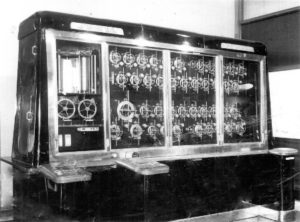
Doodson-Légé machine for forecasting the ocean tides: when it comes to complexity and transparency, we have different demands from a data analysis tool than we have from a prediction machine.
Machine learning techniques such as artificial neural networks and support vector machines are by now widely known within the tech world. In contrast, other means of data analysis like subgroup discovery and local modeling mostly remain niche methods. However, they actually have a high value proposition in diverse scenarios from business to science and thus deserve more attention. Subgroup discovery in particular is a very flexible framework that allows to easily express and effectively answer practical analysis questions. In this post, I give an intuitive introduction to this framework assuming only a mild familiarity with machine learning and data analysis. In particular, I’d like to approach the topic from a somewhat unconventional but hopefully insightful angle: the idea that in data analysis it is often surprisingly powerful to selectively say “I don’t know”.
To explain what I mean by that, let us start by differentiating two activities that can emerge around a given data collection: predictive (global) modeling where our goal is to turn the data into an as accurate as possible prediction machine and (exploratory) data analysis where we aim to automatically discover novel insights about the domain in which the data was measured.
The ultimate purpose of the first is automatization. i.e., to use a machine to substitute human cognition (e.g., for autonomously driving a car based on sensor inputs). In contrast, the purpose of the second is to use machine discoveries to synergistically boost human expertise (e.g., for understanding commonalities and differences among PET scans of Alzheimer’s patients [1]). It is this synergistic support that local modeling and pattern discovery techniques are designed for and that dictates how they trade off accuracy, complexity, and generality.
A good prediction machine does not necessarily provide explicit insights into the data domain
When building a prediction machine, we mainly care about prediction accuracy, i.e., the proximity of predicted outputs when running the model over the sample as well as previously unseen inputs. Although models with a large number of parameters, i.e., with a high complexity, need more training data to achieve a high accuracy, we happily raise the complexity when sufficient data is available. When doing this, however, the resulting models typically loose their ability to provide explicit insights into the data domain—at least not in a way that is comprehendible by a human user.
As an illustration of this phenomenon, consider the following simple example where I measured for a population of 300 data points the values of two variables, x and y. Let us refer to y as the target variable, i.e., this is the variable I want to ultimately understand. Think of “order volume” or “health after treatment”. Correspondingly, let us refer to x as a description variable, i.e., an additional measurement that I can make for members of my population that could potentially influence the target (e.g., “time spent on site” or “time of treatment”).
-
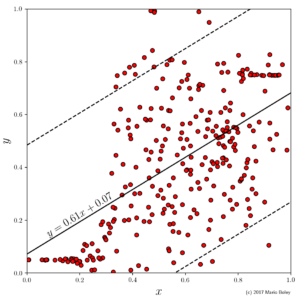
- Figure 1: example dataset 1 with global linear regression model and upper and lower 95% prediction bands (dashed lines).

-

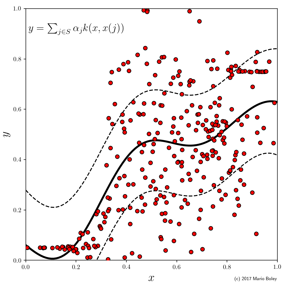
- Figure 2: dataset 1 with Gaussian process regression model and covariance band (dashed) using sum of Gaussian and noise kernel.
As a starting point, in Figure 1, I performed the perhaps most well-known data analysis technique and modeled y as a linear function of x, i.e., y=ax+b, by performing ordinary least squares regression on the sample points. While this model is simple, it is not very accurate (even on the given sample) and, hence, it allows to draw little to no conclusions about the underlying domain (y does not seem to be a linear function of x).
Our inclination in predictive modeling is now to raise the model complexity; for instance by fitting a Gaussian process model, which corresponds to a smooth function represented by a linear combination of density functions around each training data point. As we can see in Figure 2, this model improves the accuracy, but at the same time we lost the ability to say easily why a certain x value receives a certain predicted y value (it is due to the overall weighted proximity to all training examples which is represented by the 300 coefficients, \alpha_j for j=1,...,300).
A complex theory of everything might be of less value than a simple observation about a specific part of the data space
Thus, this example shows that in data analysis we have to value simplicity in its own right. At the same time, of course, we cannot neglect accuracy. So how can we solve this conundrum? The answer lies in the relaxation of the third, rather implicit, requirement mentioned above: generality. In contrast to a self-driving car, which should better propose a control action for every possible sensor input, when analyzing PET scans, we have the power to selectively focus on those parts of the input space where we see a pattern and to say ‘I don’t know’ to others.
In other words, while a predictive modeling algorithm has to find an as accurate as possible and as complex as necessary global function, a pattern discovery algorithm can report models that are only a
-
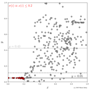
- Figure 3: subgroup discovery result consisting of point selector (red) and constant local model; dashed line indicates 95% prediction band.

-
- Figure 4: augmenting the dataset by a second descriptive feature allows to discover another subgroup using a conjunctive selector.

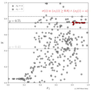
As we can see in Figure 3, the output of subgroup discovery does not only entail a model but also a selector \sigma that describes the domain of definition for that model. In our example, this selector takes on the form of a simple inequality condition on the x variable: \sigma(\cdot) \equiv x(\cdot) \leq 0.2. It turns out that, among the 19 selected data points (marked red), the y variable can be modeled accurately even by a constant function. So by sacrificing generality we were able to increase the model accuracy and the model simplicity at the same time (compared to the initial linear regression model from Figure 1). Impressive, isn’t it?
Well, keeping track of the complexity more thoroughly, we have to admit that it actually stayed more or less unchanged: for the parameter we lost by going from a linear to a constant function we gained one threshold parameter in the subgroup selector. However, the accuracy gain is real. Hence, we can note two things:
- Saying “I don’t know” to all data points i with x(i) > 0.2 allowed us to trade model generality for model accuracy.
- We have to specify carefully a language of possible selector functions that is expressive on the one hand but not too complex on the other.
A meaningful subgroup selection language is crucial for discovering interesting patterns
The second point refers to what is often called the learning bias in machine learning. Introducing a bias, i.e., limiting the ways for the subgroup discovery algorithm to select local model domains, is crucial to end up with useful patterns: if we could just select any arbitrary subset of data points, we would end up with an observation that is meaningless at best (simply sorting out all points we don’t like doesn’t make an interesting discovery) and highly misleading at worst (because it would simply vanish when sampling new data from the same domain).
It turns out that the following is a theoretically and practically reasonable scheme: For each variable that I move from the modeling to the selection space (as happened to x in our example), I can allow all possible threshold functions as basic selectors and then let my selection language contain all
This selection language has the further advantage that we can easily mix in categorical variables for good measure, i.e., variables that can take on values from a small finite and unordered set (such as \mathrm{age} \in \{\mathrm{male}, \mathrm{female}\}). For example in Figure 4, we use the categorical variable x_2 to identify another subgroup with accurate constant model through the selector x_1\geq 0.8 \wedge x_2=a. This is an advantage over many machine learning algorithms which often can either work with only numerical or only categorical variables.
Subgroups look similar to decision trees but good tree learners are forced to brush over some local structure in favor of the global picture
In fact, the subgroup selection language appears closely related to decision or regression trees. Indeed, a single subgroup is syntactically the same as a leaf in a decision or regression tree, and thus tree leafs often correspond to interesting local patterns. When fitting a tree, however, we again optimize the joint, i.e., global, accuracy of all leafs. Consequently, when limiting the complexity, we can again miss interesting local structure as the following example shows.
-
- Figure 5: example dataset 2 with categorical target variable and two numeric description variables; colored areas show decision surface of a two level deep decision tree.

-
- Figure 6: two subgroups with high accuracies can be found; both groups are not picked up by decision tree despite similar language.
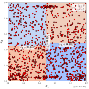
In Figure 5, I fitted a decision tree to a dataset with 975 points, one categorical target variable y, and two numeric descriptive variables x_1 and x_2. At the root node the tree splits the data according to the decision boundary x_1 \leq 0.503 (the vertical line at the center) followed for each of the two possible decisions by a second split somewhere at the middle along the x_2-axis (where the exact threshold depends on the choice in the first decision). Hence, using three conditions, we end up with a decision surface given by four rectangles of roughly equal size: the two blue areas (upper left and lower right) where the majority y-value is b as well as the two red areas (upper right and lower left) with the majority value y=a.
By predicting the majority value for each region, the tree classifies 618 out of 975 data points correctly (63.4% sample accuracy). From the perspective of the decision tree learner, i.e., from the perspective of building a global prediction machine, this tree is optimal among all 2-level trees—an improvement would just be possible by increasing the number of conditions aka the complexity. However, with our bare eye we can identify two regions, one in the lower center and one in in the upper center of the data space, which are densely populated and allow a 100% sample accuracy. In the interest of global performance, the decision tree does not only not capture these regions. In fact, it cuts right through them.
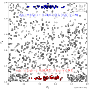
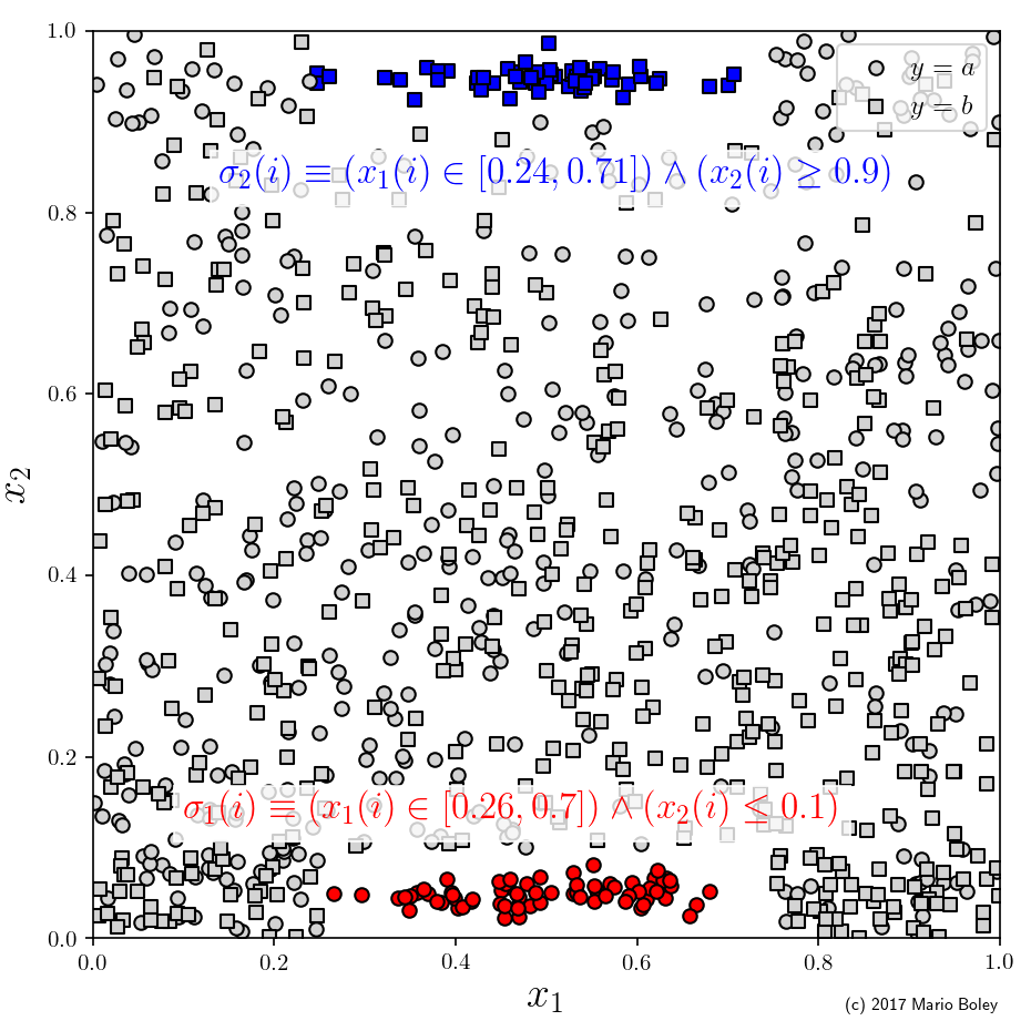
In contrast to that, as we can see in Figure 6, subgroup discovery is able to select either of these groups using the same number of conditions as the global decision tree. The first one (red) selects 70 points and the second (blue) selects 55—as stated above: each with 100% sample accuracy. In contrast, the local region of highest accuracy identified by the decision tree is the lower-right rectangle (x_1 \geq 0.486 \wedge x_2 \leq 0.483) where the majority prediction gets only 205 of 299 (or 69.7%) of the data points right.
Which of these trade-offs between accuracy and generality we prefer might of course depend on the specific application we are dealing with. Generally, however, when performing local modeling we tend to emphasize the accuracy and to treat generality as a secondary criterion that assures the statistical validity of our discoveries. This points to a second ingredient to subgroup discovery that we have to define in addition to the selection language: an objective function that determines the value of all the different subgroups that we could potentially identify in the data.
One classical choice, which is motivated from the idea of statistical validity and that yielded the above results, is the binomial test function f_{\text{bn}}(\sigma)=\sqrt{\frac{|\text{ext}(\sigma)|}{|S|}}\left(p_+(\text{ext}(\sigma))-p_+(S)\right) where |\text{ext}(\sigma)| and |S| denote the size of the selection \text{ext}(\sigma) and the complete sample S, respectively, and p_+(\text{ext}(\sigma)) and p_+(S) denote the fraction of points with the desired y-value within the selection and the complete sample, respectively.
Going one step further, we can find local trends that are opposed to the global trend
Looking at the possible options for objective functions in local modeling leads me to the final motive I’d like to discuss in this introduction: the discovery of exceptional patterns. We have already seen that local data regions can be used to find more accurate models than global models without increasing the complexity. Going one step further, we can use subgroup discovery to find local regions in the data space exhibiting trends that are opposed to the global trend.
This is a central idea of local pattern discovery, and, we have in fact already seen a motivating example for this in Figures 3 and 4 above. In both cases the local model fitted to the data was not only more accurate than the global model but also their parameter differed drastically from the global model parameter (y=0.05 and y=0.75 locally versus y=0.43 globally). The following example illustrates the same principle. At the same time it provides a glimpse beyond the simple settings of subgroup discovery we have seen so far by increasing the number of target variables from one to two (which is a relatively young idea; see [2]).
-

-
Figure 7: example dataset 3 with two numeric target variables and a single categorical description variable; lines show global linear model
between target variables.

-

- Figure 8: two subgroups can be identified that do not only have a higher accuracy but also an exceptional model slope inverse to the trend in the global data.
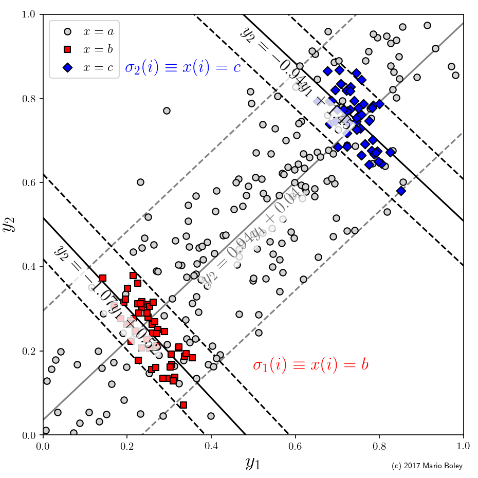
Indeed, as you can see in Figure 7, in this example we consider two numeric target variables, y_1 and y_2, in addition to one categoric descriptive variable x. Suppose we are interested in the relationship between the two target variables. We can fit a global linear model y_2=ay_1+b, which reveals a fairly accurate linear trend with a positive correlation. Surprisingly, however, there are two subgroups that can be identified through the additional variable x in which the dependency between y_1 and y_2 is reversed.
A famous setting showing such a constellation is Robinson’s paradox [3], where the connection between the fraction of foreign-born Americans (y_1) and the rate of English literacy (y_2) of the US states was investigated based on the 1930 census data. As in the example above, when looking at the global trend there seems to be a positive correlation. However, when selecting subgroups based on a state’s wealth, the connection is inverted, which is due to the fact that wealth of an area is a confounding factor: while on an individual level being foreign-born and English literacy have a negative correlation, on a geographic level, wealthy areas attract more immigrants but also have a higher literacy of the overall population.
Whether the global data inhibits an ecological fallacy as in Robinson’s paradox or the global trend is indeed valid but is inverted for certain population members (think, e.g., of patients with prior conditions that suffer adverse effects from an otherwise useful drug): subgroup discovery is capable of automatically detecting such exceptional trends in the data that deserve our attention.
Further reading…
In case you got intrigued by this short introduction to the power of saying “I don’t know”, I encourage you to look for further reading. In particular, here we only discussed the specification of a subgroup discovery problem (target and description variables, selection language, and objective function) but left entirely open how one can go about solving it.
Before I provide some pointers, let me start with a warning: the state of the field is by far not as mature as general machine learning. Peter Flach’s book [4] is the only textbook I am aware of that contains a chapter dedicated to subgroup discovery. Another more comprehensive resource is the dissertation of Wouter Duivesteijn [5]. Other than that, you are in the jungle of academic papers.
A good starting point to pave your way through that jungle is Martin Atzmüller’s survey [6] from 2015. Moreover, if you are interested specifically in subgroup discovery algorithmics, I’d like to advertise our own recent work with colleagues from MPI Informatics and the Fritz Haber Institute [7]. If you are more interested in applications: with the same authors we have also shown how subgroup discovery can be used in materials science [8]. These applications (crystal structure and electronic property prediction) also come with an interactive hands-on tutorial using Creedo.
I hope this was helpful. Don’t hesitate to drop questions/comments in the reply section below.
References
[Bibtex]
@article{schmidt2010interpreting,
title={Interpreting PET scans by structured patient data: a data mining case study in dementia research},
author={Schmidt, Jana and Hapfelmeier, Andreas and Mueller, Marianne and Perneczky, Robert and Kurz, Alexander and Drzezga, Alexander and Kramer, Stefan},
journal={Knowledge and Information Systems},
volume={24},
number={1},
pages={149--170},
year={2010},
publisher={Springer},
paperurl = {schmidt2010interpreting.pdf}
}[Bibtex] [Link]
@article{duivesteijn2016exceptional,
title={Exceptional model mining},
author={Duivesteijn, Wouter and Feelders, Ad J and Knobbe, Arno},
journal={Data Mining and Knowledge Discovery},
volume={30},
number={1},
pages={47--98},
year={2016},
publisher={Springer},
doi={10.1007/s10618-015-0403-4},
url={https://doi.org/10.1007/s10618-015-0403-4}
}[Bibtex]
@article{robinson1950ecological,
title={Ecological Correlations and the Behavior of Individuals},
author={Robinson, WS},
journal={American Sociological Review},
volume={15},
number={3},
pages={351--357},
year={1950},
publisher={JSTOR}
}[Bibtex]
@book{flach2012machine,
title={Machine learning: the art and science of algorithms that make sense of data},
author={Flach, Peter},
year={2012},
publisher={Cambridge University Press}
}[Bibtex]
@phdthesis{duivesteijn2013exceptional,
title={Exceptional model mining},
author={Duivesteijn, Wouter},
year={2013},
school={Leiden Institute of Advanced Computer Science (LIACS), Faculty of Science, Leiden University}
}[Bibtex] [Link]
@article{atzmueller2015subgroup,
title={Subgroup discovery},
author={Atzmueller, Martin},
journal={Wiley Interdisciplinary Reviews: Data Mining and Knowledge Discovery},
volume={5},
number={1},
pages={35--49},
year={2015},
publisher={Wiley Online Library},
doi={10.1002/widm.1144},
url={http://onlinelibrary.wiley.com/doi/10.1002/widm.1144/epdf}
}[Bibtex] [Paper] [Slides] [Link]
@article{boley2017identifying,
author="Boley, Mario
and Goldsmith, Bryan R.
and Ghiringhelli, Luca M.
and Vreeken, Jilles",
title="Identifying consistent statements about numerical data with dispersion-corrected subgroup discovery",
journal="Data Mining and Knowledge Discovery",
year="2017",
month="Jun",
day="28",
doi="10.1007/s10618-017-0520-3",
}[Bibtex] [Paper] [Link]
@article{goldsmith2017uncovering,
title={Uncovering structure-property relationships of materials by subgroup discovery},
author={Goldsmith, Bryan R and Boley, Mario and Vreeken, Jilles and Scheffler, Matthias and Ghiringhelli, Luca M},
journal={New Journal of Physics},
volume={19},
number={1},
pages={013--031},
year={2017},
publisher={IOP Publishing},
doi={10.1088/1367-2630/aa57c2}
}| a. | ↑ | The precise sense of complexity here is the VC-dimension, which is connected to the generalization error or to how reliable we can measure the accuracy of a result based on its performance on the given data sample. |